https://en.wikipedia.org/wiki/Benders_decomposition
Benders decomposition - Wikipedia
From Wikipedia, the free encyclopedia Jump to navigation Jump to search Benders decomposition (or Benders' decomposition) is a technique in mathematical programming that allows the solution of very large linear programming problems that have a special bloc
en.wikipedia.org
연구실 친구가 쓴 위키피디아 글인데 공부할 겸 일부 번역해서 정리하고 일부 설명이 미흡하다고 생각한 부분의 설명을 추가했다. 원문 전체를 커버하지는 않으니 원문과 같이 공부에 활용하시는게 좋을듯. (이해 안되는 설명이 있다면 댓글 달아주세요~ 틀린 내용이 있다면 지적 환영하고 디스커션 환영합니다. )
개요
Benders decomposition 이란 divide-and-conquer 전략의 일종으로 큰 LP 문제를 여러개의 블록으로 쪼갤 수 있게 해준다. 원래 문제의 변수들은 두개의 subset 으로 나뉜다. first-stage master problem은 첫번째 subset 에 있는 변수 y 들의 값을 구해낸다. 첫번째 단계에서 결정된 y 값을 고정한 상태에서 second-stage subproblem 에서는 두번째 subset 에 있는 x 변수들의 값을 결정한다. 그 후 두번째 단계에서의 결과 값을 바탕으로 master problem 을 수정해나가는 iterative 한 과정을 거친다. 구체적으로 어떻게 master problem을 수정해 나가는지 아래에서 알아보자.

Mathematical formulation

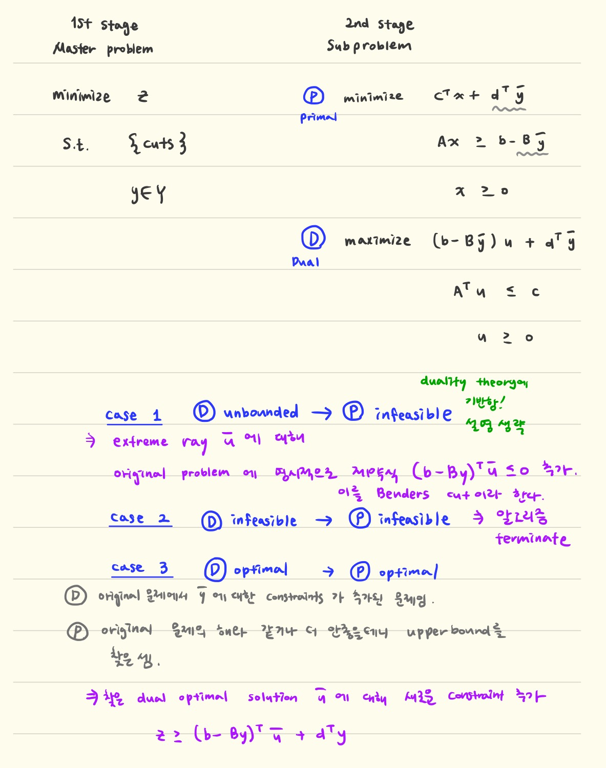
앞서 개요에서 설명했듯 Benders decomposition은 큰 LP 문제를 Master problem 과 subproblem으로 나누고 master problem에서 구한 y를 고정한 상태에서 subproblem 의 해를 구해낸다. 위에 전개된 수식은 original problem 과 decomposed 된 문제가 수학적으로 equivalent 하다는 것을 보여준다.
Iteration process
맨 처음 master problem은 cuts 이 empty 인 상태에서 출발한다. cut 은 constraint 에 대응된다. (constraints 가 만드는 convex set 을 떠올려보면 constraint 하나가 공간을 구분하는 선분/면 에 대응되므로 cut 이라고 표현하는 의미를 알 수 있다.) 처음에는 아무런 제약조건이 없으니 lower bound, upper bound 각각이 -inf, inf 로 설정된 셈이다. 이 lower bound 와 upper bound의 차이가 epsilon 보다 작아지거나 optimal solution이 없다는 certificate (이 부분 이해 안되면 duality theory 따로 공부해야함!) 을 찾게 되었을때 알고리즘을 종결한다.
알고리즘이 시작할때 y는 아무거나 feasible 하기만 한 값을 찾는 식으로 first guess를 한다. master problem 에서 y 값을 찾았으면 이를 고정하고 subproblem으로 넘어간다. subproblem 의 해는 세가지 가능성을 갖는다.
첫번째, subproblem의 dual 최적해가 unbounded 일 수 있다. duality theory 에 의해 이 경우 primal 문제는 infeasible 하다. original problem 에 benders cut을 더해준다. (위 노트 보라색 글씨 참고)
두번째, subproblem 의 dual 최적해가 infeasible 하면 알고리즘은 종결된다.
세번째, subproblem 의 dual 최적해를 찾으면 그건 primal 의 최적해와 같다. 다만 여기서는 y-bar 에 대한 제약식이 추가된 문제를 풀었다는 사실을 기억하자. lower bound를 찾은 셈이고 z값의 lower bound를 제약식으로 더해준다. (위 노트 보라색 글씨 참고)
결국 첫번째 두번째 케이스에서는 optimal solution 이 없다는 certificate 인 u-bar을 찾은 셈이고 이 경우 알고리즘을 종결한다.
세번째 케이스에서는 upper bound를 찾은 셈이며 master problem에 새로운 constraint 를 추가하는 식으로 upper bound를 명시적으로 반영해준다. 새로운 제약식이 추가된 master problem 을 다시 풀면 feasible solution 을 구할 수 있는데, 이는 lower bound 가 될 것이다. (master problem은 original problem 에서 constraint 를 몇개 뺀 문제이고 optimality 를 일정 부분 포기한 문제를 푼 셈이므로 master problem 의 objective value 는 original problem의 lower bound 가 된다.) 이렇게 업데이트 된 lower bound, upper bound의 차이가 epsilon 보다 작다면 알고리즘을 종결하고, 아니라면 next iteration 으로 넘어가서 알고리즘 종결 조건을 만족할때 까지 iteration 한다.
정리하며
Benders decomposition이 해를 향해 나아가기 위해 계속해서 새로운 constraints를 더해 나가기 때문에 row generation 이라고 부르기도 한다. 이와 대비되는 것이 Dantzig-Wolfe의 decomposition 기법인 column generation 가 있다.
'석박사 > 최적화는 사기가 아니얏!' 카테고리의 다른 글
| Column Generation 과 Dantzig-Wolfe Decomposition (0) | 2022.07.19 |
|---|---|
| [Gurobi] big-M constraint 가 일으킬 수 있는 문제 (0) | 2021.11.23 |
| ILP 문제를 푸는 exact method (cutting plane, branch-and-bound, branch-and-cut) (0) | 2021.11.05 |
| TSP 연구에 사용할만한 솔버와 예제 문제 (0) | 2021.10.13 |
| [최적화 솔버] Google ortools 와 GUROBI (0) | 2021.06.20 |

